Multivariate Distributions

Learning Goals

Know what a joint distribution of a two or more random variables is (continuous or discrete).
Know how to compute probabilities, as well as marginals and conditional distributions of joint distributions.
Understand what it means for two random variables to be independent and how to test it.

Introduction

In real life, you will most often be interested in data that has multiple values of interest in an experiment. In probabilistic language, this means you are interested in the outcome of two or more random variables at the same time. The goal of this is often to deduce some kind of relationship (or lack thereof) between the data (this can be measured using the notions of covariance and correlation which we will discuss in the next lecture).

For example, you might be interested in:

Number of Coronavirus deaths and the average age of a population
The number of posts per day and the number of followers of Instagram users
The frequency of exercise and the academic performance of college students
The salary and gender of a population in a country

Question

How do you expect that the two variables in the above examples are related? Can you think of any other pairs of random variables that you might be interested in?

Another situation where we are often interested in multiple random variables is when conducting repeated experiments that have some variability. In this case (assuming the experiment is done correctly) the outcomes of each experiment should be independent in that the outcome of one experiment shouldn't affect the outcome of the next (we will discuss in more detail what it means for two random variables to be independent in later on in these notes). In fact we have been dealing with multiple independent random variables already in the setting of the law of large numbers and the central limit theorem (something that we will comeback to later).

Joint Distributions

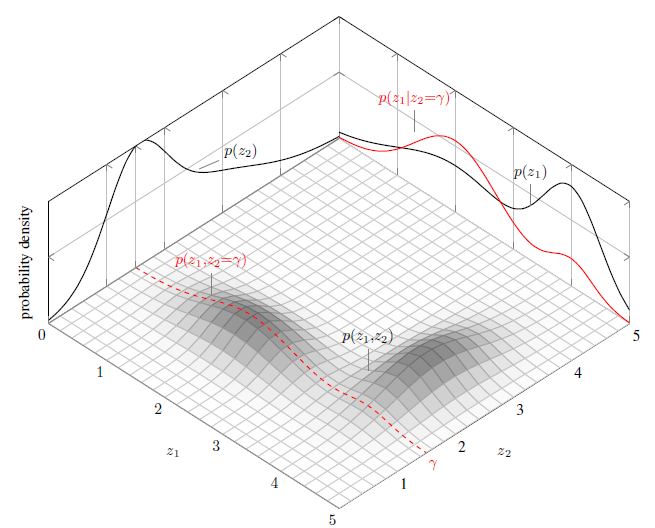
When dealing with multiple random variables, say $X, Y$ it is important to understand how they are they are distributed together. Since it is possible that $X$ can depend on $Y$ , the statistics of $(X, Y)$ can reveal behavior that simply studying the statistics of $X$ or $Y$ alone cannot.

Discrete Case

Lets start with the case when the random variables are discrete. We first introduce the idea of a joint probability distribution which describes how both $X$ and $Y$ are distributed.

Joint probability distribution

Let

X

and

Y

be two discrete random variables, then the joint probability distribution of

X

and

Y

is given by

p (x, y) := P (X = x, Y = y), where x, y \in R .

Since $X$ and $Y$ are discrete (and can therefore only take on a finite or countable number of values), the joint distribution $p (x, y)$ is only non-zero at a countable number of values.

Note

Knowing the distributions of $X$ and $Y$ separately is generally not enough to determine the joint distribution of $X$ and $Y$ (unless they are independent as we will see later). As we will see, the joint distribution $p (x, y)$ contains information about how the random variables $X$ and $Y$ depend on one another.

Suppose that $X$ takes values ${x_{1}, x_{2}, \dots, x_{n}}$ and $Y$ takes values ${y_{1}, y_{2}, \dots y_{m}}$ . Then the pair $(X, Y)$ takes values ${(x_{1}, y_{1}), (x_{2}, y_{2}), \dots (x_{n}, y_{m})}$ . The joint distribution $p (x_{i}, y_{j})$ can be organized into a joint probability table.

$X ∖ Y$	$y_{1}$	$y_{2}$	$\dots$	$y_{m}$
$x_{1}$	$p (x_{1}, y_{1})$	$p (x_{1}, y_{2})$	$\dots$	$p (x_{1}, y_{m})$
$x_{2}$	$p (x_{2}, y_{1})$	$p (x_{2}, y_{2})$	$\dots$	$p (x_{2}, y_{m})$
$⋮$	$\dots$	$\dots$	$\dots$	$\dots$
$x_{n}$	$p (x_{n}, y_{1})$	$p (x_{n}, y_{2})$	$\dots$	$p (x_{n}, y_{m})$

Properties

Joint probability distributions must satisfy the following properties

$0 \leq p (x, y) \leq 1$ for all $x, y$ .
All the probabilities add up to one $\sum_{x} \sum_{y} p (x, y) = 1,$ where the sum is over all values $x, y$ such that $p (x, y) \neq 0$ .

Note: The above summation is over a discrete set of values since $X$ and $Y$ are discrete. It can be an infinite sum.

Lets consider some examples:

Example 1 (Roll two fair dice)

Recall from the notes on discrete probability the problem of rolling two fair dice. Let

X = outcome of die 1 Y = outcome of die 2,

then the probability table is given by:

$X ∖ Y$	1	2	3	4	5	6
1	$\frac{1}{36}$	$\frac{1}{36}$	$\frac{1}{36}$	$\frac{1}{36}$	$\frac{1}{36}$	$\frac{1}{36}$
2	$\frac{1}{36}$	$\frac{1}{36}$	$\frac{1}{36}$	$\frac{1}{36}$	$\frac{1}{36}$	$\frac{1}{36}$
3	$\frac{1}{36}$	$\frac{1}{36}$	$\frac{1}{36}$	$\frac{1}{36}$	$\frac{1}{36}$	$\frac{1}{36}$
4	$\frac{1}{36}$	$\frac{1}{36}$	$\frac{1}{36}$	$\frac{1}{36}$	$\frac{1}{36}$	$\frac{1}{36}$
5	$\frac{1}{36}$	$\frac{1}{36}$	$\frac{1}{36}$	$\frac{1}{36}$	$\frac{1}{36}$	$\frac{1}{36}$
6	$\frac{1}{36}$	$\frac{1}{36}$	$\frac{1}{36}$	$\frac{1}{36}$	$\frac{1}{36}$	$\frac{1}{36}$

Since there are $36$ cells in the table, the total probability clearly sums up to one.

This table is pretty boring since it does not indicate an interesting relationship between the random variables $X$ , and $Y$ . In fact $X$ and $Y$ are independent.

As a more interesting case, consider another random variable $Z = 7 - X,$ which takes what ever $X$ gives and "flips" it around 3. Then $X$ and $Z$ are clearly dependent, since the value of $X$ completely determines the value of $Z$ , the probability table becomes:

$X ∖ Z$	1	2	3	4	5	6
1	0	0	0	0	0	1/6
2	0	0	0	0	1/6	0
3	0	0	0	1/6	0	0
4	0	0	1/6	0	0	0
5	0	1/6	0	0	0	0
6	1/6	0	0	0	0	0

If you were to look at the distribution of just $Z$ , you wouldn't be able to tell that $Z$ was "copying" off of $X$ . This can only be recognized by considering the joint distribution.

We can also consider more complicated events.

Example 2

Let $X$ and $Y$ be as in the previous example. What is the probability that $X < Y$ ?

The event ${X < Y}$ can be described explicitly as the set of $(x, y)$ pairs

\begin{aligned} {X < Y} = { & (1, 2), (1, 3), (1, 3), (1, 5), (1, 6), \\ (2, 3), (2, 4), (2, 4), (2, 5), (2, 6), \\ (3, 4), (3, 5), (3, 6), \\ (4, 5), (4, 6), (5, 6)} . \end{aligned}

This can be visualized as a triangular subset of the probability table considered in Example 1, colored salmon below:

$X ∖ Y$	1	2	3	4	5	6
1	$\frac{1}{36}$	$\frac{1}{36}$	$\frac{1}{36}$	$\frac{1}{36}$	$\frac{1}{36}$	$\frac{1}{36}$
2	$\frac{1}{36}$	$\frac{1}{36}$	$\frac{1}{36}$	$\frac{1}{36}$	$\frac{1}{36}$	$\frac{1}{36}$
3	$\frac{1}{36}$	$\frac{1}{36}$	$\frac{1}{36}$	$\frac{1}{36}$	$\frac{1}{36}$	$\frac{1}{36}$
4	$\frac{1}{36}$	$\frac{1}{36}$	$\frac{1}{36}$	$\frac{1}{36}$	$\frac{1}{36}$	$\frac{1}{36}$
5	$\frac{1}{36}$	$\frac{1}{36}$	$\frac{1}{36}$	$\frac{1}{36}$	$\frac{1}{36}$	$\frac{1}{36}$
6	$\frac{1}{36}$	$\frac{1}{36}$	$\frac{1}{36}$	$\frac{1}{36}$	$\frac{1}{36}$	$\frac{1}{36}$

Since there are $15$ such elements, we see that $P (X < Y) = \frac{15}{36} .$

The concept of joint probability can easily be generalized to the case of $n$ random variables

Multivariate joint probability function

Let $X_{1}, X_{2}, \dots X_{n}$ be discrete random variables, then the joint probability distribution of $X_{1}, X_{2}, \dots X_{n}$ is given by

p (x_{1}, x_{2}, \dots, x_{n}) := P (X_{1} = x_{1}, X_{2} = x_{2}, \dots X_{n} = x_{n}) .

where

(x_{1}, x_{2}, \dots, x_{n}) \in R^{n}

. Again, since

X_{1}, X_{2}, \dots X_{n}

are discrete,

p (x_{1}, x_{2}, \dots x_{n})

can only be non-zero on at most a discrete set of values.

Of course we must still, have $0 \leq p (x_{1}, x_{2}, \dots, x_{n}) \leq 1$ , and $\sum_{x_{1}, x_{2}, \dots, x_{n}} p (x_{1}, x_{2}, \dots, x_{n}) = 1$ where the sum is over all values of $(x_{1}, x_{2}, \dots x_{n})$ such that $p (x_{1}, x_{2}, \dots, x_{n}) \neq 0$ .

Continuous Case

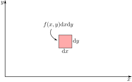
To treat two continuous random variables, $X$ and $Y$ . We start by analogy with the single variable case. Namely instead of evaluating probabilities at specific values, we must evaluate probabilities on subsets of $R^{2}$ . In this case, we can think of the probability distribution as being given by the the infinitesimal probability associated to some joint probability density $f (x, y)$ (or joint pdf)

In general we can describe probabilities for $X$ and $Y$ using multivariable calculus and area integrals.

Joint probability density

Let

X

Y

be two continuous random variables, then the joint probability density function

f (x, y)

X

and

Y

is defined by

\begin{matrix} (1) & P ((X, Y) \in R) = \iint_{R} f (x, y) d A . \end{matrix}

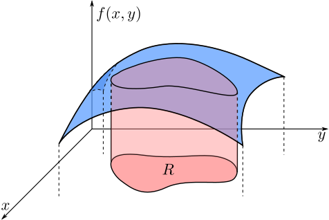
The integral in $(1)$ is an area integral and can be approximated by a sum $\iint_{R} f (x, y) d A \approx \sum_{i j} f (x_{i}, y_{j}) Δ x_{i} Δ y_{j}$ of volumes of rectangular prisms each with volume $f (x_{i}, y_{j}) Δ x_{i} Δ y_{j}$ . We can interpret $p (i, j) = f (x_{i}, y_{j}) Δ x_{i} Δ y_{j}$ as a joint probability distribution function associated to the rectangle centered around $(x_{i}, y_{j})$ .

Just as with the single variable case, a joint probability density must satisfy non-negativity and normality.

Properties

A joint probability density $f (x, y)$ for two continuous random variables $X$ and $Y$ must satisfy

$0 \leq f (x, y)$ for all $x, y \in R$ .
The total integral is 1, $\int_{0}^{\infty} \int_{0}^{\infty} f (x, y) d x d y = 1.$

Computing Double Integrals (a review)

The area integral in the definition $(1)$ , can be calculated by iterated integrals if $R$ can be cleanly described in certain coordinates.

Rectangular coordinates:If $R$ is the rectangle $R = [a, b] \times [c, d]$ , then we have

P ((X, Y) \in R) = \int_{a}^{b} (\int_{c}^{d} f (x, y) d y) d x .

Depending, on $f (x, y)$ , the integral can then be computed by first freezing $x$ , integrating $y$ and then integrating $x$ (or vice-versa). See the iterated integral section of Paul's Online Notes for a refresher on how to do this as well as some examples.

Regions bounded by functions: If $R$ is a more general region bounded between two curves $g_{1} (x) \leq g_{2} (x)$ so that

R = {(x, y) \in R^{2} : a \leq x \leq b, g_{1} (x) \leq y \leq g_{2} (x)},

then we can write the iterated integral like

P ((X, Y) \in R) = \int_{a}^{b} \int_{g_{1} (x)}^{g_{2} (x)} f (x, y) d y d x .

See the Integration over General Regions sections of Paul's Online Notes for a refresher on how to do this as well as some examples.

Polar coordinates: As another example if the region $R$ is a circle $R = {x^{2} + y^{2} \leq 1}$ , then the area integral can be written as an iterated polar integral

P ((X, Y) \in R) = \int_{0}^{2 π} (\int_{0}^{1} f (r \cos θ, r \sin θ) r d r) d θ .

See the Integrals in Polar Coordinates sections of Paul's Online Notes for a refresher on how to do this as well as some examples.

Example 3

Suppose that $X$ and $Y$ are continuous random variables with values in $[0, 1]$ and joint density given by $f (x, y) = {\begin{cases} c x y, & if 0 \leq x, y \leq 1 \\ 0 & otherwise \end{cases}$

What is the value of $c$ that makes this a valid joint pdf? For this value of $c$ , what is the probability that $X > 1 / 2$ and $Y < 1 / 2$ ?

Clearly $f (x, y) \geq 0$ , if $c \geq 0$ , and therefore we simply need to check the normality condition 2. We can do this using iterated partial integrals:

\begin{aligned} \int_{- \infty}^{\infty} \int_{- \infty}^{\infty} c x y d x d y & = \int_{0}^{1} \int_{0}^{1} c x y d x d y \\ = \int_{0}^{1} {(\frac{c}{2} x^{2} y]}_{x = 0}^{x = 1} d y = \int_{0}^{1} \frac{c}{2} y d y \\ = {(\frac{c}{4} y^{2}]}_{0}^{1} = \frac{c}{4} . \end{aligned}

Therefore we need $c = 4$ for this to be a valid joint pdf.

To find the probability that $X > 1 / 2$ and $Y < 1 / 2$ we note that

{X > 1 / 2, Y < 1 / 2} = {(X, Y) \in [1 / 2, 1] \times [0, 1 / 2]} .

Therefore the iterated integral can be set up as

\begin{aligned} P (X > \frac{1}{2}, Y < \frac{1}{2}) & = \int_{0}^{\frac{1}{2}} \int_{\frac{1}{2}}^{1} 4 x y d x d y \\ = \int_{0}^{\frac{1}{2}} {(2 y x^{2}]}_{x = 1 / 2}^{x = 1} d y \\ = \int_{0}^{\frac{1}{2}} 2 y (1 - \frac{1}{4}) d y \\ = \frac{1}{4} (\frac{3}{4}) = \frac{3}{16} . \end{aligned}

Lets consider a more complicated joint density defined over a different shaped region.

Example 4 (Triangular Region)

This problem is taken from Example 5.4 in the text.

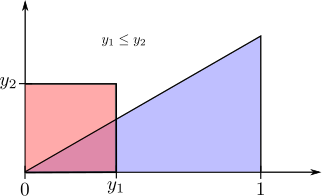
Suppose that $Y_{1}$ and $Y_{2}$ are continuous random variables with values in $[0, 1]$ such that $Y_{2} \leq Y_{1}$ and the joint density given by $f (x, y) = {\begin{cases} c y_{1}, & if 0 \leq y_{2} \leq y_{1} \leq 1 \\ 0 & otherwise \end{cases}$

What is the value $c$ that makes $f (y_{1}, y_{2})$ a valid joint density function? What is the probability that $0 \leq Y_{1} \leq 1 / 2$ and $Y_{2} > 1 / 4$ ?

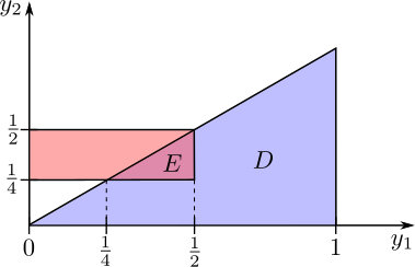
Let's check the normality condition. First, we should recognize that the domain of $f (y_{1}, y_{2})$ is a triangular region (shown in the figure below)

D = {(y_{1}, y_{2}) \in R^{2} : 0 \leq y_{1} \leq 1, 0 \leq y_{2} \leq y_{1} \leq 1}

This is a region bounded between two curves and there integral can be set up as

\begin{aligned} \int_{0}^{1} \int_{0}^{y_{1}} c y_{1} d y_{2} d y_{1} & = \int_{0}^{1} c y_{1} {(y_{2}]}_{0}^{y_{1}} d y_{1} \\ = \int_{0}^{1} c y_{1}^{2} d y_{1} = \frac{c}{3} = 1. \end{aligned}

Therefore we must have $c = 3$ .

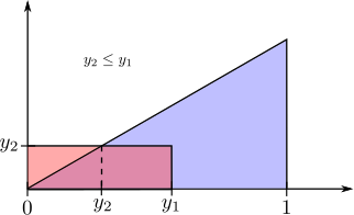
To compute the probability that $0 \leq Y_{1} \leq 1 / 2$ and $Y_{2} > 1 / 4$ we need to carefully consider the region we are integrating over. Note, for instance, that if $Y_{1} < 1 / 4$ , then since $Y_{2} \leq Y_{1}$ , it's not possible for $Y_{2} \geq 1 / 4$ . We need to consider how the region ${0 \leq y_{1} \leq 1 / 2, y_{2} > 1 / 4}$ overlaps with the triangular domain $D = {0 \leq y_{2} \leq y_{1} \leq 1}$ . This is illustrated in the following figure.

As we can see, the event of interest is

E = {(y_{1}, y_{2}) : \frac{1}{4} \leq y_{1} \leq \frac{1}{2}, \frac{1}{4} \leq y_{2} \leq y_{1}} .

The associated integral is

\begin{aligned} P ((Y_{1}, Y_{2}) \in E) & = \int_{\frac{1}{4}}^{\frac{1}{2}} \int_{\frac{1}{4}}^{y_{1}} 3 y_{1} d y_{2} d y_{1} \\ = \int_{\frac{1}{4}}^{\frac{1}{2}} 3 y_{1} (y_{1} - \frac{1}{4}) d y_{1} \\ = {(y_{1}^{3} - \frac{3}{8} y_{1}^{2}]}_{\frac{1}{4}}^{\frac{1}{2}} \\ = \frac{5}{128} . \end{aligned}

Of course this can all be extended in a straight-forward way to the case of $n$ jointly distributed random variables. However, this is beyond the scope of this course.

Multivariate joint probability density (optional)

Let $X_{1}, X_{2}, \dots X_{n}$ be continuous random variables, then the joint pdf, $f (x_{1}, x_{2}, \dots, x_{n})$ , of $X_{1}, X_{2}, \dots X_{n}$ is define in terms of the $n$ -dimensional volume integral

P ((X_{1}, X_{2}, \dots X_{n}) \in R) = \int \int \dots \int_{R} f (x_{1}, \dots, x_{n}) d V,

where $R \subset R^{n}$ is any subregion of $n$ dimensional space. In this setting, it is useful to think of $X = (X_{1}, X_{2}, \dots, X_{n})$ as a random $n$ -dimensional vector in.

Joint Cumulative Distribution

As was the case with single random variables, the distribution of probability between two discrete or continuous random variables can be characterized by the joint cumulative distribution function (or joint cdf)

Joint cumulative distribution

For any two random variables

X, Y

, the joint cumulative distribution function is defined by

F (x, y) := P (X \leq x, Y \leq y) .

Note: that this is defined regardless of whether

X, Y

are discrete or continuous.

This can be written in terms of the joint distribution of joint density in the discrete or continuous cases.

Discrete case

If $X$ and $Y$ are discrete random variables with joint distribution function $p (x, y)$ , then the joint cdf is just given by

F (x, y) = \sum_{u \leq x} \sum_{v \leq y} p (u, v),

where the sum is over $u$ and $v$ such that $p (u, v) \neq 0$ .

Example 5

Let $X$ and $Y$ be as in the previous example be as in example 1. What is $F (3.5, 4)$ ?

$F (3.5, 4)$ is just the event $X \leq 3.5, Y \leq 4$ , we can visualize this shading cells in the probability table, colored salmon below:

$X ∖ Y$	1	2	3	4	5	6
1	$\frac{1}{36}$	$\frac{1}{36}$	$\frac{1}{36}$	$\frac{1}{36}$	$\frac{1}{36}$	$\frac{1}{36}$
2	$\frac{1}{36}$	$\frac{1}{36}$	$\frac{1}{36}$	$\frac{1}{36}$	$\frac{1}{36}$	$\frac{1}{36}$
3	$\frac{1}{36}$	$\frac{1}{36}$	$\frac{1}{36}$	$\frac{1}{36}$	$\frac{1}{36}$	$\frac{1}{36}$
4	$\frac{1}{36}$	$\frac{1}{36}$	$\frac{1}{36}$	$\frac{1}{36}$	$\frac{1}{36}$	$\frac{1}{36}$
5	$\frac{1}{36}$	$\frac{1}{36}$	$\frac{1}{36}$	$\frac{1}{36}$	$\frac{1}{36}$	$\frac{1}{36}$
6	$\frac{1}{36}$	$\frac{1}{36}$	$\frac{1}{36}$	$\frac{1}{36}$	$\frac{1}{36}$	$\frac{1}{36}$

Since there are $12$ such elements, we see that $F (3.5, 4) = \frac{12}{36} .$

Continuous case

If $X$ and $Y$ are continuous random variables with joint pdf $f (x, y)$ , then the joint cdf is just given by

F (x, y) = \int_{- \infty}^{x} \int_{- \infty}^{y} f (u, v) d v d u .

We can also recover the joint pdf from the joint cdf using partial derivatives $f (x, y) = \frac{\partial^{2} F}{\partial x \partial y} (x, y) .$

Example 6

Let $Y_{1}$ and $Y_{2}$ be as in Example 4. What is the joint cdf?

The event $Y_{1} \leq y_{1}$ and $Y_{2} \leq y_{2}$ depends on whether $y_{1} \leq y_{2}$ or $y_{1} \geq y_{2}$ . Both cases are illustrated below

If $0 \leq y_{1} \leq y_{2} \leq 1$ , then the region of integration is a triangle

\begin{aligned} F (y_{1}, y_{2}) & = \int_{0}^{y_{1}} \int_{0}^{t_{1}} 3 t_{1} d t_{2} d t_{1} \\ = \int_{0}^{y_{1}} 3 t_{1}^{2} d t_{1} \\ = y_{1}^{3} \end{aligned}

On the other hand, if $0 \leq y_{2} \leq y_{1} \leq 1$ then the region of integration can be split up into a triangle and rectangle

\begin{aligned} F (y_{1}, y_{2}) & = \int_{0}^{y_{2}} \int_{0}^{t_{1}} 3 t_{1} d t_{2} d t_{1} + \int_{y_{2}}^{y_{1}} \int_{0}^{y_{2}} 3 t_{1} d t_{2} d t_{1} . \\ = y_{2}^{3} + \int_{y_{2}}^{y_{1}} 3 t_{1} y_{2} d t_{1} \\ = y_{2}^{3} + \frac{3}{2} (y_{1}^{2} - y_{2}^{2}) y_{2} \\ = - \frac{1}{2} y_{2}^{3} + \frac{3}{2} y_{1}^{2} y_{2} . \end{aligned}

Putting this together gives

F (y_{1}, y_{2}) = {\begin{cases} y_{1}^{3} & if 0 \leq y_{1} \leq y_{2} \leq 1 \\ - \frac{1}{2} y_{2}^{3} + \frac{3}{2} y_{1}^{2} y_{2} & if 0 \leq y_{2} \leq y_{1} \leq 1 \\ 1 & if y_{1} \geq 1 and y_{2} \geq 1 \\ 0 & otherwise \end{cases} .

As was the case in one dimension, the joint cdf has various properties

Properties of the joint cdf

If $X$ and $Y$ are any random variables with joint cdf $F (x, y)$ then the following properies hold

F(x,y) is non-decreasing, meaning that if $x$ or $y$ increase, then $F (x, y)$ can't decrease
If you send any variable to $- \infty$ , then $F (x, y)$ goes to zero, i.e. $F (- \infty, - \infty) = F (- \infty, y) = F (x, - \infty) = 0.$
If you send both variables to $+ \infty$ , then $F (x, y)$ approaches $1$ , i.e. $F (\infty, \infty) = 1$ .

Using the cdf to calculate probabilities of rectangles

Just like in the single variable case, the cdf can be used to calculate probabilities on rectangles. This can be stated more precisely as: if $x_{1} \geq x_{2}$ and $y_{1} \geq y_{2}$ , then the following rule holds.

P (x_{1} \leq X \leq x_{2}, y_{1} \leq Y \leq y_{2}) = F (x_{2}, y_{2}) - F (x_{2}, y_{1}) - F (x_{1}, y_{2}) + F (x_{1}, y_{1})

This is illustrated in the following animation using the additive and subtractive properties of probability. Positive contributions are colored red and negative contributions are colored blue.

Marginal distributions

If two random variables $X$ and $Y$ are jointly distributed, it is often the case that you want to understand the distribution just one of them, ignoring any relationship between the two of them, such a distribution is called a marginal distribution.

Discrete case

Lets begin by considering an example:

Example 7

Recall the die tossing experiment from Example 1. Suppose we consider the event ${X = 3}$ . We know that this corresponds to the the following pairs

{X = 3} = {(3, 1), (3, 2), (3, 3), (3, 4), (3, 5), (3, 6)} .

This corresponds to row

3

in the table.

$X ∖ Y$	1	2	3	4	5	6
1	$\frac{1}{36}$	$\frac{1}{36}$	$\frac{1}{36}$	$\frac{1}{36}$	$\frac{1}{36}$	$\frac{1}{36}$
2	$\frac{1}{36}$	$\frac{1}{36}$	$\frac{1}{36}$	$\frac{1}{36}$	$\frac{1}{36}$	$\frac{1}{36}$
3	$\frac{1}{36}$	$\frac{1}{36}$	$\frac{1}{36}$	$\frac{1}{36}$	$\frac{1}{36}$	$\frac{1}{36}$
4	$\frac{1}{36}$	$\frac{1}{36}$	$\frac{1}{36}$	$\frac{1}{36}$	$\frac{1}{36}$	$\frac{1}{36}$
5	$\frac{1}{36}$	$\frac{1}{36}$	$\frac{1}{36}$	$\frac{1}{36}$	$\frac{1}{36}$	$\frac{1}{36}$
6	$\frac{1}{36}$	$\frac{1}{36}$	$\frac{1}{36}$	$\frac{1}{36}$	$\frac{1}{36}$	$\frac{1}{36}$

Using the additive law of probability, we can calculate $P (X = 3)$ by summing along the rows of the table

P (X = 3) = p (3, 1) + p (3, 2) + p (3, 3) + p (3, 4) + p (3, 5) + p (3, 6) = \frac{1}{6} .

Of course we already knew this!

Motivated by the example, we define marginal distributions

Marginal probability distribution

Suppose that $X$ and $Y$ are discrete random variables with joint distribution function $p (x, y)$ . The marginal distribution functions $p_{X} (x)$ and $p_{Y} (y)$ for $X$ and $Y$ respectively are given by summing the joint distribution over the other variable

p_{X} (x) := \sum_{y} p (x, y), p_{Y} (y) := \sum_{x} p (x, y),

where the sum's are over all values such that

p (x, y) \neq 0

The marginals can be visualized in the following extension of the joint probability table, where the sums of each row and column are located on the right and bottom margins.

$X ∖ Y$	$y_{1}$	$y_{2}$	$\dots$	$y_{m}$	$p_{X} (x)$
$x_{1}$	$p (x_{1}, y_{1})$	$p (x_{1}, y_{2})$	$\dots$	$p (x_{1}, y_{m})$	$p_{X} (x_{1})$
$x_{2}$	$p (x_{2}, y_{1})$	$p (x_{2}, y_{2})$	$\dots$	$p (x_{2}, y_{m})$	$p_{X} (x_{2})$
$⋮$	$\dots$	$\dots$	$\dots$	$\dots$	$⋮$
$x_{n}$	$p (x_{n}, y_{1})$	$p (x_{n}, y_{2})$	$\dots$	$p (x_{n}, y_{m})$	$p_{X} (x_{n})$
$p_{Y} (y)$	$p_{Y} (y_{1})$	$p_{Y} (y_{2})$	$\dots$	$p_{Y} (y_{m})$	$1$

Note

The marginal distributions say very little about a joint distribution. Two random variables can have the same marginal distribution and be very dependent on one another. For instance if $X$ is the outcome of a fair die roll, then $Z = 7 - X$ has the same marginal distribution as $X$ even though $Z$ is completely determined by the outcome of $X$ .

Continuous Case

The continuous case is similar to the discrete case, where sums are replaces with integrals.

Marginal probability density

Suppose that $X$ and $Y$ are continuous random variables with joint pdf $f (x, y)$ . The marginal distribution pdfs $f_{X} (x)$ and $f_{Y} (y)$ for $X$ and $Y$ respectively are given by integrating out the other variable.

f_{X} (x) := \int_{- \infty}^{\infty} f (x, y) d y, f_{Y} (y) := \int_{- \infty}^{\infty} f (x, y) d x .

Example 8

Consider the joint pdf from Example 3

f (x, y) = {\begin{cases} 4 x y & if 0 \leq x, y, \leq 1 \\ 0 & otherwise \end{cases}

Find the $X$ and $Y$ marginals.

To find

f_{X} (x)

we integrate out the

y

variable and to find

f_{Y} (y)

we integrate out the

x

variable.

f_{X} (x) = \int_{0}^{1} 4 x y d y = {[2 x y^{2}]}_{0}^{1} = 2 x

f_{Y} (y) = \int_{0}^{1} 4 x y d x = {[2 x^{2} y]}_{0}^{1} = 2 y .

Example 9

Consider the more complicated pdf of Example 4

f (y_{1}, y_{2}) = {\begin{cases} 3 y_{1} & if 0 \leq y_{2} \leq y_{1} \leq 1 \\ 0 & otherwise \end{cases}

Find the $X$ and $Y$ marginals.

Taking into account the triangular region,

f_{Y_{1}} (y_{1}) = \int_{0}^{y_{1}} 3 y_{1} d y_{2} = 3 y_{1}^{2}

f_{Y_{2}} (y_{2}) = \int_{y_{2}}^{1} 3 y_{1} d y_{1} = \frac{3}{2} (1 - y_{2}^{2}) .

Marginal cdf

Finding the marginal cdf from a given joint cdf is actually pretty easy. No integration or summation is necessary.

Marginal cdf

Let $X$ and $Y$ be two random variables with joint cdf $F (x, y)$ , then the marginal cdfs are given by

F_{X} (x) = lim_{y \to \infty} F (x, y), F_{Y} (y) = lim_{x \to \infty} F (x, y) .

Note that if $X$ and $Y$ only take values in a rectangle $[a, b] \times [c, d]$ , then this can be simplified to evaluating $x$ or $y$ at the right end point of it's respective domain,

F_{X} (x) = F (x, d), F_{Y} (y) = F (b, y) .

Lets illustrate this ideas with a more complicated example.

Example 10

Lets consider the cdf we calculated from Example 6.

F (y_{1}, y_{2}) = {\begin{cases} y_{1}^{3} & if 0 \leq y_{1} \leq y_{2} \leq 1 \\ - \frac{1}{2} y_{2}^{3} + \frac{3}{2} y_{1}^{2} y_{2} & if 0 \leq y_{2} \leq y_{1} \leq 1 \\ 1 & if y_{1} \geq 1 and y_{2} \geq 1 \\ 0 & otherwise \end{cases} .

Find the $X$ and $Y$ marginal cdfs.

Evaluating at the $y_{1} = 1$ and $y_{2} = 1$ gives

F_{Y_{1}} (y_{1}) = F (y_{1}, 1) = y_{1}^{3}

F_{Y_{2}} (y_{2}) = F (1, y_{2}) = \frac{1}{2} (3 y_{2} - y_{2}^{3}) .

Note that $F_{Y_{1}}^{'} (y_{1}) = 3 y_{1}^{2}$ and $F_{Y_{2}}^{'} (y_{2}) = \frac{3}{2} (1 - y_{2}^{2})$ , which is consistent with the answers to Example 9.

Conditional Distributions

In addition to marginal distributions, one can also define conditional distributions that describe the distribution of one random variable given the value of another.

Discrete case

Recall the definition of conditional probability of $A$ given $B$ .

P (A | B) = \frac{P (A \cap B)}{P (B)} .

We can apply this formula to the distribution of two discrete random variables $X$ and $Y$ , using the random variables to define events like ${X = 1}$ and ${Y = 2}$ . Then we can consider the probability $X$ taking a certain value given that $Y$ takes a different value by

P (X = 1 | Y = 2) = \frac{P (X = 1, Y = 2)}{P (Y = 2)} .

This motivates the following definition.

Conditional distribution function

Let $X$ and $Y$ be two random variables with joint distribution $p (x, y)$ , then the conditional distribution function of $X$ given $Y$ is

p (x | y) := \frac{p (x, y)}{p_{Y} (y)},

provided that

p_{Y} (y) \neq 0

. A similar definition holds for

p (y | x)

p (y | x) := \frac{p (x, y)}{p_{X} (x)},

Note

$p (x | y)$ is undefined if $p_{Y} (y) = 0$ . This is because it doesn't make sense to condition on a probability zero event.

Continuous case

The continuous case is much more subtle. For instance, it is hard to define $P (X \leq x | Y = y),$ since the probability that ${Y = y}$ is zero.

However, one of the remarkable features of continuous probability distributions is that it is possible to make sense of conditioning on ${Y = y}$ by taking a limit. For instance, we can define a conditional cdf by shrinking the interval $[y, y + h]$ to the point $y$ and defining

P (X \leq x | Y = y) := lim_{h \to 0} P (X \leq x | y \leq Y \leq y + h) .

The next result shows that this limit exists and

Conditional cdf

Let $X$ and $Y$ be two continuous random variables with joint pdf $f (x, y)$ and joint cdf $F (x, y)$ , then the conditional cdf of $X$ given $Y$ is defined by

\begin{aligned} F (x | y) & := lim_{h \to 0} P (X \leq x | y \leq Y \leq y + h) \\ = \frac{\partial_{y} F (x, y)}{f_{Y} (y)} = \frac{\int_{0}^{x} f (u, y) d u}{f_{Y} (y)} \end{aligned}

provided that

f_{Y} (y) \neq 0

Proof:

The expression $P (X \leq x | y \leq Y \leq y + h)$ is well defined since $P (y \leq Y \leq y + h) \neq 0$ for some values of $y$ .

We can calculate this limit explicitly since

\begin{aligned} P (X \leq x | y \leq Y \leq y + h) & = \frac{P (X \leq x, y \leq Y \leq y + h)}{P (y \leq Y \leq y + h)} \\ = \frac{F (x, y + h) - F (x, y)}{F_{Y} (y + h) - F_{Y} (y)} \\ = \frac{\frac{1}{h} (F (x, y + h) - F (x, y))}{\frac{1}{h} (F_{Y} (y + h) - F_{Y} (y))}, \end{aligned}

where in the last line we multiplied and divided by $\frac{1}{h}$ . Using the fact that

\frac{1}{h} (F (x, y + h) - F (x, y)) \to \partial_{y} F (x, y) = \int_{0}^{x} f (u, y) d u

\frac{1}{h} (F_{Y} (y + h) - F_{Y} (y)) \to F_{Y}^{'} (y) = f_{Y} (y),

as $h \to 0$ , completes the proof.

QED

This motivates the following definition of the conditional pdf by taking the derivative of the conditional cdf.

Conditional pdf

Let $X$ and $Y$ be two continuous random variables with joint pdf $f (x, y)$ , then the conditional pdf of $X$ given $Y$ is

f (x | y) := \partial_{x} F (x | y) = \frac{f (x, y)}{f_{Y} (y)},

provided that

f_{Y} (y) \neq 0

. An analogous definition holds for

f (y | x)

Example 11

Lets consider pdf from Example 6.

f (y_{1}, y_{2}) = {\begin{cases} 3 y_{1} & if 0 \leq y_{2} \leq y_{1} \leq 1 \\ 0 & otherwise \end{cases}

Find $f (y_{1} | y_{2})$ and use it to calculate $P (Y_{1} \leq 3 / 4 | Y_{2} = 1 / 2)$ .

From example 9, we found that $f_{Y_{2}} (y_{2}) = \frac{3}{2} (1 - y_{2}^{2}) 0 \leq y_{2} \leq 1.$ Therefore

f (y_{1} | y_{2}) = {\begin{cases} \frac{2 y_{1}}{1 - y_{2}^{2}} & if 0 \leq y_{2} \leq y_{1} \leq 1 \\ 0 & otherwise . \end{cases}

To calculate $P (Y_{1} \leq 1 / 2 | Y_{2} = 1 / 2)$ we note that

f (y_{1} | 1 / 2) = {\begin{cases} \frac{8}{3} y_{1} & if \frac{1}{2} \leq y_{1} \leq 1 \\ 0 & otherwise . \end{cases}

Therefore

\begin{aligned} P (Y_{1} \leq 3 / 4 | Y_{2} = 1 / 2) & = \int_{0}^{3 / 4} f (y_{1} | 1 / 2) d y_{1} \\ = \int_{1 / 2}^{3 / 4} \frac{8}{3} y_{1} d y_{1} \\ = \frac{4}{3} (\frac{9}{16} - \frac{1}{4}) \\ = \frac{5}{12} \end{aligned}

Independence of Random Variables

We can now give a precise definition of independence of two random variables.

Recall that two events $A$ and $B$ are independent if and only if $P (A \cap B) = P (A) P (B) .$ Of course we can take $A$ and $B$ to be events defined to two random variables $X$ and $Y$ , for instance $A = {X \leq 3}$ and $B = {Y \geq 1}$ . We then say that two random variables $X$ and $Y$ are independent if any event defined by $X$ and any event defined by $Y$ are independent. As it turns out it's good enough to consider events of the form ${X \leq x}$ and ${Y \leq y}$ for all $x$ and $y$ , the condition $P (X \leq x, Y \leq y) = P (X \leq x) P (Y \leq y)$ guarantees independence.

Independence

Two random variables $X$ and $Y$ with joint cdf $F (x, y)$ and marginal cdfs $F_{X} (x)$ and $F_{Y} (y)$ are independent if and only if

F (x, y) = F_{X} (x) F_{Y} (y) .

Otherwise $X$ and $Y$ are said to be dependent.

In the discrete case, the definition can be reduced to:

Independence (discrete case)

Two discrete random variables $X$ and $Y$ with joint distribution function $p (x, y)$ and marginal distributions $p_{X} (x)$ and $p_{Y} (y)$ are independent if and only if

p (x, y) = p_{X} (x) p_{Y} (y) .

Otherwise $X$ and $Y$ are said to be dependent.

In the discrete case, independence means the probability in a cell of the probability table must be the product of the marginal probabilities of its row and column. This is considered in the next example.

Example 12

Lets consider the die rolling experiment from Example 1. Of course we know that $X$ and $Y$ are independent, but lets check that out notion of independence is correct.

The probability table is

$X ∖ Y$	1	2	3	4	5	6	$p_{X} (x)$
1	$\frac{1}{36}$	$\frac{1}{36}$	$\frac{1}{36}$	$\frac{1}{36}$	$\frac{1}{36}$	$\frac{1}{36}$	$\frac{1}{6}$
2	$\frac{1}{36}$	$\frac{1}{36}$	$\frac{1}{36}$	$\frac{1}{36}$	$\frac{1}{36}$	$\frac{1}{36}$	$\frac{1}{6}$
3	$\frac{1}{36}$	$\frac{1}{36}$	$\frac{1}{36}$	$\frac{1}{36}$	$\frac{1}{36}$	$\frac{1}{36}$	$\frac{1}{6}$
4	$\frac{1}{36}$	$\frac{1}{36}$	$\frac{1}{36}$	$\frac{1}{36}$	$\frac{1}{36}$	$\frac{1}{36}$	$\frac{1}{6}$
5	$\frac{1}{36}$	$\frac{1}{36}$	$\frac{1}{36}$	$\frac{1}{36}$	$\frac{1}{36}$	$\frac{1}{36}$	$\frac{1}{6}$
6	$\frac{1}{36}$	$\frac{1}{36}$	$\frac{1}{36}$	$\frac{1}{36}$	$\frac{1}{36}$	$\frac{1}{36}$	$\frac{1}{6}$
$p_{Y} (y)$	$\frac{1}{6}$	$\frac{1}{6}$	$\frac{1}{6}$	$\frac{1}{6}$	$\frac{1}{6}$	$\frac{1}{6}$	1

Since each marginal has probability $\frac{1}{6}$ and each cell has probability $\frac{1}{36}$ (the produce of the marginals), we can see that $X$ and $Y$ are independent.

On the otherhand, lets consider $X$ and $Z = 7 - X$ . The probability table was given by

$X ∖ Z$	1	2	3	4	5	6	$p_{X} (x)$
1	0	0	0	0	0	$\frac{1}{6}$	$\frac{1}{6}$
2	0	0	0	0	$\frac{1}{6}$	0	$\frac{1}{6}$
3	0	0	0	$\frac{1}{6}$	0	0	$\frac{1}{6}$
4	0	0	$\frac{1}{6}$	0	0	0	$\frac{1}{6}$
5	0	$\frac{1}{6}$	0	0	0	0	$\frac{1}{6}$
6	$\frac{1}{6}$	0	0	0	0	0	$\frac{1}{6}$
$p_{Z} (z)$	$\frac{1}{6}$	$\frac{1}{6}$	$\frac{1}{6}$	$\frac{1}{6}$	$\frac{1}{6}$	$\frac{1}{6}$	1

In this table, we can see that many of the probabilities are not the product of two marginal probabilities and so $X$ and $Z$ are dependent. Indeed, since none of the marginal probabilities are zero, then none of the cells with zero probability can be a product of marginals.

In the continuous case (by taking partial derivatives), this can be reduced to a statement on the pdfs:

Independence (continuous case)

Two continuous random variables $X$ and $Y$ with joint pdf $f (x, y)$ and marginal pdfs $f_{X} (x)$ and $f_{Y} (y)$ are independent if and only if

f (x, y) = f_{X} (x) f_{Y} (y) .

Otherwise $X$ and $Y$ are said to be dependent.

In many ways the continuous case is easier to check that the discrete case, since it can be reduced to showing that the density can be factored into a product of two densities.

Example 13

Let

X

and

Y

have joint density

f (x, y) = {\begin{cases} 4 x y & if 0 \leq x, y \leq 1 \\ 0 & otherwise \end{cases}

Are

X

and

Y

independent?

In this case, since $f_{X} (x) = 2 x$ for $0 \leq x \leq 1$ and $f_{Y} (y) = 2 y$ and $0 \leq y \leq 1$ , we can easily see that for $0 \leq x, y \leq 1$ , $f_{X} (x) f_{Y} (y) = 4 x y = f (x, y) .$

Example 14

How about the pdf from Example 6? Are $Y_{1}$ and $Y_{2}$ independent?

In this case, we know that for $0 \leq y_{1} \leq 1$ and $0 \leq y_{2} \leq 1$ we have

f_{Y_{1}} (y_{1}) = 3 y_{1}^{2}, f_{Y_{2}} (y_{2}) = \frac{3}{2} (1 - y_{2}^{2}) .

So that for all $0 \leq y_{1}, y_{2} \leq 1$

f_{Y_{1}} (y_{1}) f_{Y_{2}} (y_{2}) = \frac{9}{2} y_{1}^{2} (1 - y_{2}^{2}) .

This is no where close to $f (y_{1}, y_{2})$ if not for the simple fact that $f_{Y_{1}} (y_{1}) f_{Y_{2}} (y_{2}) \neq 0$ when $0 \leq y_{1} \leq y_{2} \leq 1$ while $f (y_{1}, y_{2}) = 0$ .

Notes APMA 1650 - Spring 2020

Multivariate Distributions

Learning Goals

Introduction

Question

Joint Distributions

Discrete Case

Note

Example 1 (Roll two fair dice)

Example 2

Continuous Case

Computing Double Integrals (a review)

Example 3

Example 4 (Triangular Region)

Joint Cumulative Distribution

Example 5

Example 6

Using the cdf to calculate probabilities of rectangles

Marginal distributions

Discrete case

Example 7

Note

Continuous Case

Example 8

Example 9

Marginal cdf

Example 10

Conditional Distributions

Discrete case

Note

Continuous case

Example 11

Independence of Random Variables

Example 12

Example 13

Example 14

Notes
APMA 1650 - Spring 2020