For example, a single Stokeslet of strength
where the smooth regularizing functions  and and  satisfy satisfy |

|
 ,
,
 , so that the far field velocity is that of the
standard Stokeslet (where
, so that the far field velocity is that of the
standard Stokeslet (where
 ). In fact, for
 ,
,
 .
.
The velocity expression can also be inverted to find the forces that impose a given velocity boundary condition. The wide applicability of the method and its properties are demonstrated throught numerical examples. Solutions converge with second-order accuracy when forces are exerted along smooth boundaries. Examples of segmented boundaries and forcing at random points are also presented in the paper.
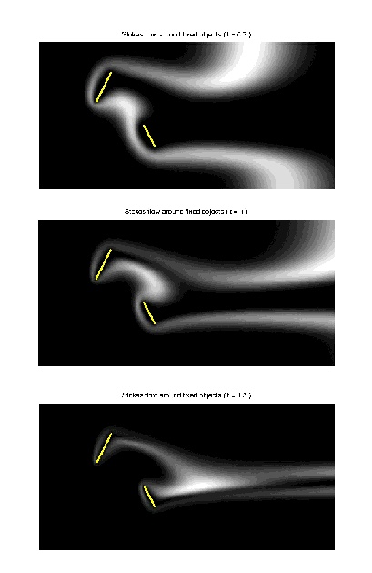
The figures on the left show a simulation of a background flow from left to right moving around two line obstacles. Given the background flow, the Method of Regularized Stokeslet is used to compute the forces along the obstacles which will identially cancel the incoming flow. As a result, the velocity of the boundary points is nearly zero (approximately 10-14, the tolerance of the iterative method used to solve for the forces).
Once the forces are known, the velocity at any point can be computed as the sum of the Stokeslet flow due to the forces and the background flow. Using this formula, the (steady) velocity was precomputed on a grid and used to advect a "cloud of white smoke" shown in the figures. The three snap shots show the smoke at three different instants of the motion.
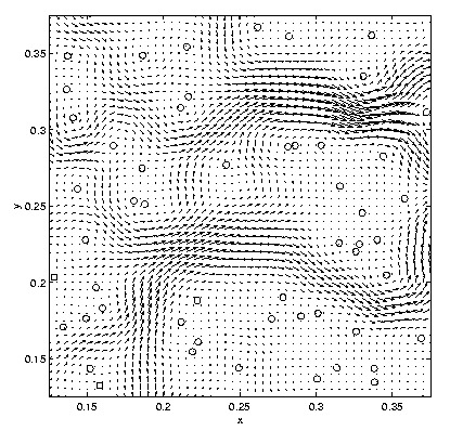
The same method can be used to compute a flow that must go around a collection of particles located at random points. Forces at the particle locations are computed so that they cancel the background flow at those locations.
The figure on the right shows 53 particles that may represent a dilute suspension or a porous medium. The vector field shows the direction of the flow as it moves around the obstacles.